A New Chapter In The True Density of Microstructures

How mastering imaging artifacts has allowed 200-year-old physics to launch density measurements into the 21st century

Contact Sales

Back to Blogs

Jeffrey Wong

Senior Application Scientist

June 24, 2026

2 Minute Read

Today, we peel back the curtains on our patented true density analysis. Despite being a fundamental material property, true density has actually historically been a challenge to measure when material microstructures are present. Our new patented density measurement method leverages high-res imaging to calculate true material density while accounting for internal microstructure. Here’s how it’s done:

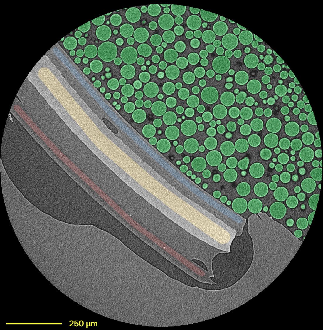
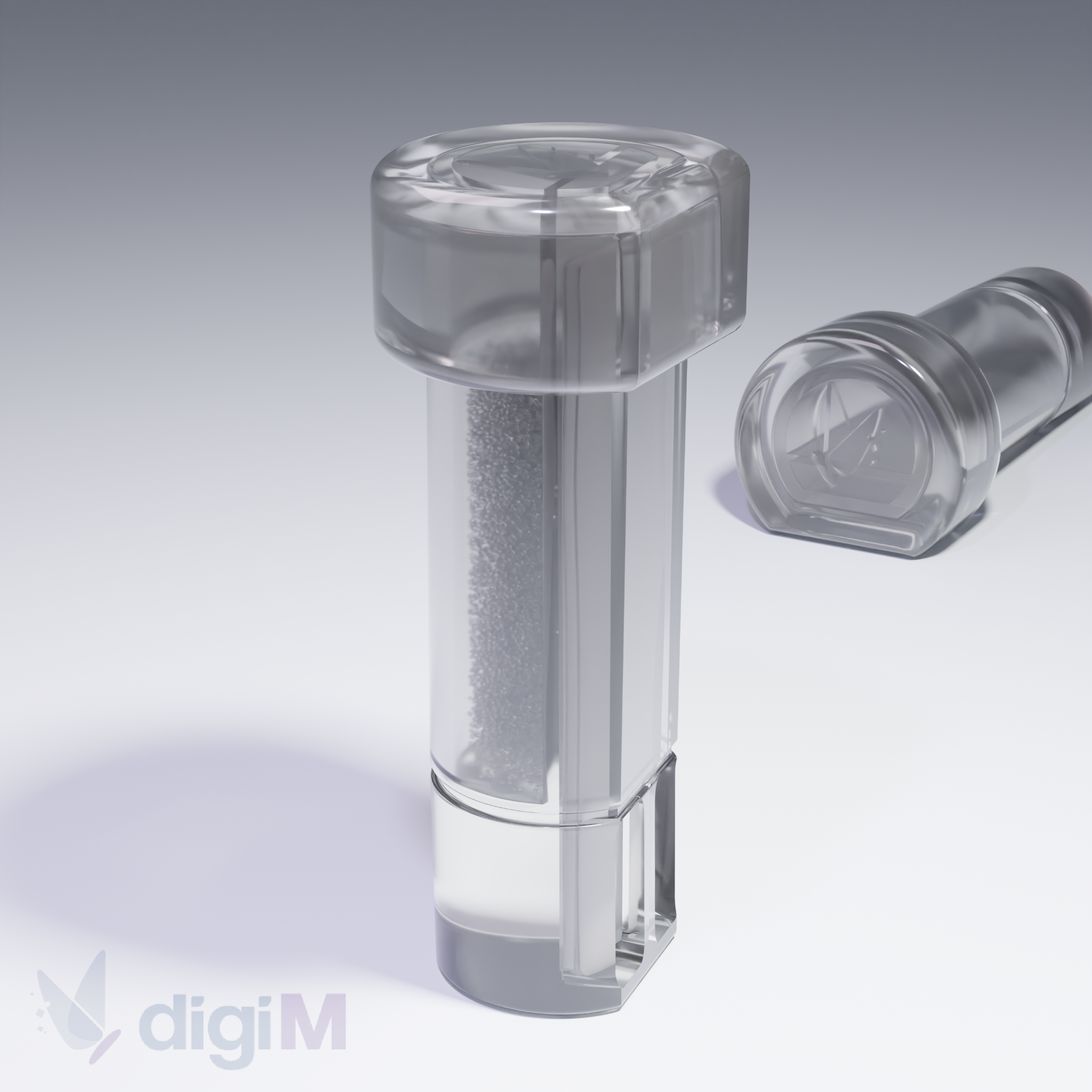
First, we need to scan our sample. Our samples are scanned inside our very own custom 3D printed sample holders, which allow us to neatly package the sample alongside a stack of pure plastic calibrants. These calibrants will provide reference density values for the next step.

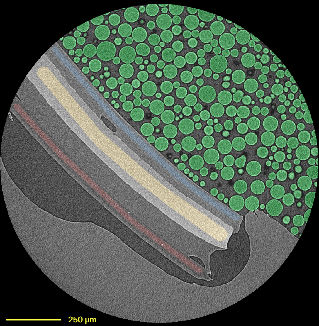
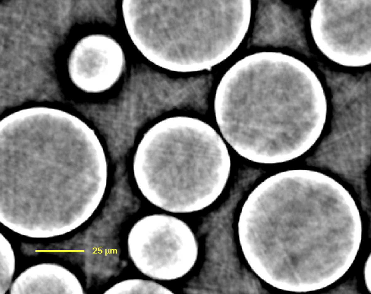
*Figure 1. Digital rendering of the sample holders digiM uses for calculating density. Actual height ~1cm.*

Once the images make their way to our analysts, they receive segmentations just like the one shown below. This not only opens the door to the measurement of density on a per-particle basis, but even allows the measurement to be refined to specific sub-regions, or mapped across an entire monolithic object such as an implant or a tablet.

Figure 2. A test sample which we’ve scanned and segmented in preparation for density calculation. The sample is labeled in green, while red, yellow, and blue are the calibrant stack. For best results, we’re only sampling the interior region of each calibrant.

To extract our precious density data, we must think back to high school and apply Beer’s Law to our image. This is why we made sure to put calibrants of known density in our sample holder. Unfortunately for us though, the laws of physics demand their dues all the same, and at this scale that means Fresnel diffraction artifacts throughout our image, which is no good for density measurement.

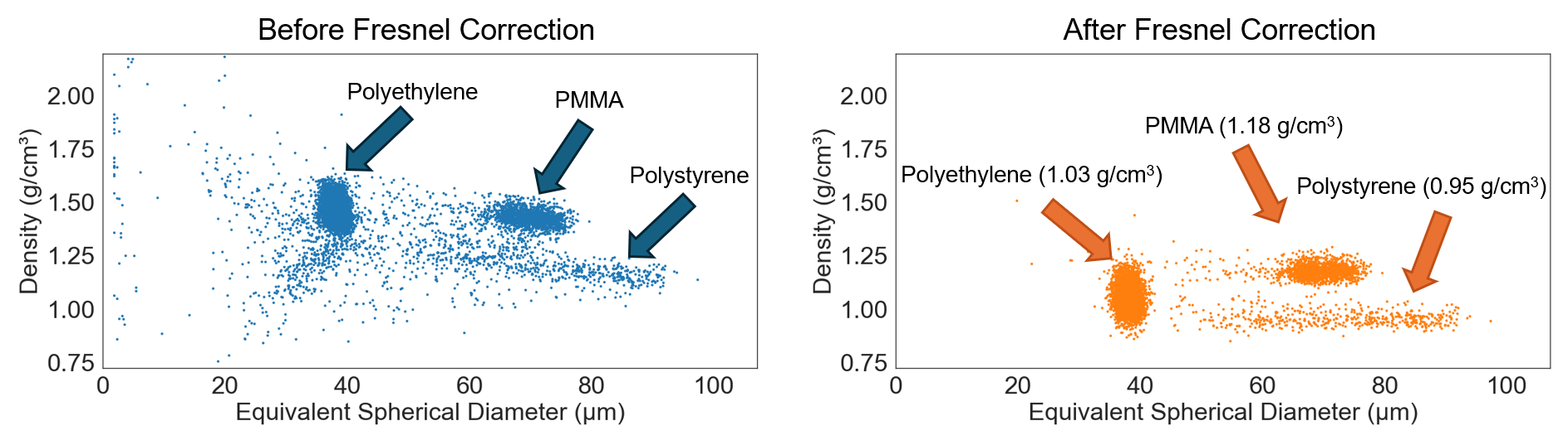
*Figure 3. A close-up look at the dreaded Fresnel artifact. Notice the bright fringe around the edge of each bead.*

Solving this issue is what finally led to our breakthrough in dialing in the accuracy of our density measurements. Our density measurement method calculates the true material brightness by removing the Fresnel artifact, giving clean, accurate results every time. And hey presto, you’ve got your density! If this all sounds too good to be true, check out one of our validation results below, where we analyzed a mixture of polystyrene, polyethylene, and PMMA beads. Each scatter point represents an individual bead in the sample, with the left and right plots highlighting the power of Fresnel artifact removal. Each of the 3 types of beads is visible as its own cluster in the plot. These are the actual results for the sample from Figure 2. Take another look and see if you can tell the different beads apart by eye. (Spoiler - you can’t!)